Chapter 4 Vegetation Analysis
4.1 Plot Data Schema
Several vegnasis functions require data frames with a predefined standard set of column names to operate.
The pre.fill.veg() was designed to allow the user to process any data frame by filter out extraneous data columns and append any missing columns. Prior to using this function, steps are initially taken to manually assign existing data to a standardized column names as much as possible. User has a responsibility to convert any legacy units of measure to SI (metric system) for subsequent analyses to be scaled properly. Conversions to USC units, if desired, should take place only as a final step after analysis.
The clean.veg() function can read the column names as they exist in NASIS and make the appropriate assignments and unit conversions.
plot = Unique identifer for plot.
label = Convenient contextual name for plot.
symbol = USDA PLANTS symbol.
taxon = Species (binomial), and sometimes genus, subspecies, or varieties.
type = Growth habit or form such as ‘tree’, ‘shrub/vine’, ‘grass/grasslike’, ‘forb’, ‘moss’, etc.
nativity = ‘native’ or ‘introduced’ status within the geographic area or the plot.
cover = crown or canopy cover (not the same as foliar cover).
stratum.min = minimum height range (m) of stratum considered to be occupied by this taxon.
stratum.max = maximum height range (m) of stratum considered to be occupied by this taxon.
crown.min = bottom height (m) of live canopy for members of this taxon occupying this stratum.
crown.max = top height (m) of live canopy for members of this taxon occupying this stratum.
dbh.min = minimum diameter (cm) of trees measured (usually at “breast height”, 1.37 or 1.4 m above the grown, a.k.a. ‘DBH’).
dbh.max = maximum diameter (cm) of trees measured (usually at “breast height”, 1.37 or 1.4 m above the grown, a.k.a. ‘DBH’). Mean diameter (cm) of all trees measured using a variable radius plot (BA prism) is the same as quadratic mean diameter of all trees within a fixed plot.
BA = basal area (square meters per hectare). In lieu of the complete set of diameters, the maximum and minimum diameter can be used to estimate the quadratic mean diameter, which is used to determine stand density with basal area.
library(vegnasis)
obsite <- c('plot1','plot1','plot1', 'plot2', 'plot2')
 obsspp <- c('Acer rubrum','Pinus strobus','Pteridium aquilinum', 'Lindera benzoin', 'Trillium grandiflorum')
 abund <- c(80,10,30,10,10)
 mydata <- data.frame(obsite=obsite, obsspp=obsspp, abund=abund)

 #Identify columns containing data corresponding to standard column names.
 mydata <- mydata |> mutate(taxon=obsspp, cover=abund, plot=obsite)
 veg <- mydata |> pre.fill.veg()

 knitr::kable(
  head(veg, 10), booktabs = TRUE,
  caption = 'A table of rudimentary veg data.'
)| plot | label | date | lat | lon | symbol | taxon | type | habit | nativity | cover | stratum.min | stratum.max | crown.min | crown.max | dbh.min | dbh.max | BA | crshape | crfill | crcolor | stshape | stfill | stcolor |
|---|---|---|---|---|---|---|---|---|---|---|---|---|---|---|---|---|---|---|---|---|---|---|---|
| plot1 | NA | NA | NA | NA | NA | Acer rubrum | NA | NA | NA | 80 | NA | NA | NA | NA | NA | NA | NA | NA | NA | NA | NA | NA | NA |
| plot1 | NA | NA | NA | NA | NA | Pinus strobus | NA | NA | NA | 10 | NA | NA | NA | NA | NA | NA | NA | NA | NA | NA | NA | NA | NA |
| plot1 | NA | NA | NA | NA | NA | Pteridium aquilinum | NA | NA | NA | 30 | NA | NA | NA | NA | NA | NA | NA | NA | NA | NA | NA | NA | NA |
| plot2 | NA | NA | NA | NA | NA | Lindera benzoin | NA | NA | NA | 10 | NA | NA | NA | NA | NA | NA | NA | NA | NA | NA | NA | NA | NA |
| plot2 | NA | NA | NA | NA | NA | Trillium grandiflorum | NA | NA | NA | 10 | NA | NA | NA | NA | NA | NA | NA | NA | NA | NA | NA | NA | NA |
4.2 Missing Data
Several function in vegnasis were created to fill in missing data in either a NASIS import, or a user constructed data set. In many cases, there is a data frame and a vector version of the same function, depending on whether there is “.df” suffix.
fill.hts.df()
- Function consolidates recorded plant height data and fills in missing values based on taxon or growth habit depending on what type of height data is missing. This function requires a data frame with standardized column names.
fill.nativity.df()
- This function fills in missing nativity data based taxon status across broad regions of North America. Taxon may still be introduced (or adventive) within a state in that region, but native considering the area collectively. If a region is not specified, the default is the nativity across the United States. This version of the function take a vegetation plot data frame (cleaned by the clean.veg function) as input.
fill.taxon.from.symbols()
- This function fills in missing plant names from USDA symbols if they exist.
fill.type.df()
- Lookup the NASIS life form “type” according to default growth habit of each taxon. Include column of existing types if existing types are to be preserved while filling in only missing values. Output is a vector that can be used to populate the plant “type”” column.
fill.usda.symbols()
- This function fills in missing USDA PLANTS symbols, assuming that the concept behind the names being used are not misapplied homonyms (auct non). If existing symbols are provided (optional), priority is given to existing symbols, while only missing data is replaced.
# remotes::install_github("phytoclast/vegnasis", dependencies = FALSE)
veg <- veg |> fill.type.df() |> fill.hts.df() |> fill.nativity.df() |> mutate(symbol = fill.usda.symbols(taxon))

 knitr::kable(
  head(veg, 10), booktabs = TRUE,
  caption = 'A table of rudimentary veg data.'
)| plot | label | date | lat | lon | symbol | taxon | type | habit | nativity | cover | stratum.min | stratum.max | crown.min | crown.max | dbh.min | dbh.max | BA | crshape | crfill | crcolor | stshape | stfill | stcolor | ht.min | ht.max | taxon.max | stand.max |
|---|---|---|---|---|---|---|---|---|---|---|---|---|---|---|---|---|---|---|---|---|---|---|---|---|---|---|---|
| plot1 | NA | NA | NA | NA | ACRU | Acer rubrum | tree | NA | native | 80 | NA | NA | NA | NA | NA | NA | NA | NA | NA | NA | NA | NA | NA | 0 | 0 | 30.0 | 0 |
| plot1 | NA | NA | NA | NA | PIST | Pinus strobus | tree | NA | native | 10 | NA | NA | NA | NA | NA | NA | NA | NA | NA | NA | NA | NA | NA | 0 | 0 | 60.0 | 0 |
| plot1 | NA | NA | NA | NA | PTAQ | Pteridium aquilinum | forb | NA | native | 30 | NA | NA | NA | NA | NA | NA | NA | NA | NA | NA | NA | NA | NA | 0 | 0 | 2.0 | 0 |
| plot2 | NA | NA | NA | NA | LIBE3 | Lindera benzoin | shrub/vine | NA | native | 10 | NA | NA | NA | NA | NA | NA | NA | NA | NA | NA | NA | NA | NA | 0 | 0 | 4.0 | 0 |
| plot2 | NA | NA | NA | NA | TRGR4 | Trillium grandiflorum | forb | NA | native | 10 | NA | NA | NA | NA | NA | NA | NA | NA | NA | NA | NA | NA | NA | 0 | 0 | 0.2 | 0 |
4.3 Aggregating Cover
Appendix K in the USNVC (FGDC (2008)) presents a formula intended to combine cover values of multiple strata without exceeding 100%.
\[C_i = (1 - \prod_{j=1}^n(1-\frac{cover_j}{100}))*100\] This is useful for many operations when combining strata or aggregating structure within a stratum. When assessing total canopy cover for a stand, individual cover values may sum greater than 100%, yet an independent assessment of cover doesn’t exceed 100%. Conversely, amount of open sky (not filtered by a crown outline) cannot be negative. More simply stated as a formula that can be plugged into RStudio:
## [1] 28## [1] 71.272Whereas a simple sum is similar to the formula when adding two small values and exceeds 100% with adding more or higher values:
## [1] 30## [1] 105The formula allows for random crown overlap, which is minimal at low density, but increases with density as total aggregated cover approaches 100%. As such, the function vegnasis::cover.agg() is used within many different functions that combine species or stratum cover.
But in reality, crowns in the same stratum avoid each other, and cover in the understory tends to correlate with gaps (avoiding shade).
The effect of crown overlap versus competition is illustrated when considering a stand of trees and treating each tree as an independent species. For and area of 16 ha (400 by 400 m), 1500 trees with crown diameters of 10 m have a potential to cover 73.6% of the area. If planted at random and allowed to overlap, about 52.1% of the area is predicted by the formula, close to a simulated value of 52.0%.
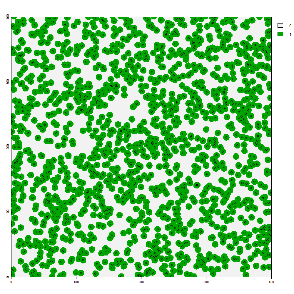
However, if an equidistant hexagonal grid is established which gives priority to planting trees further apart, the total cover does not aggree with the formula.
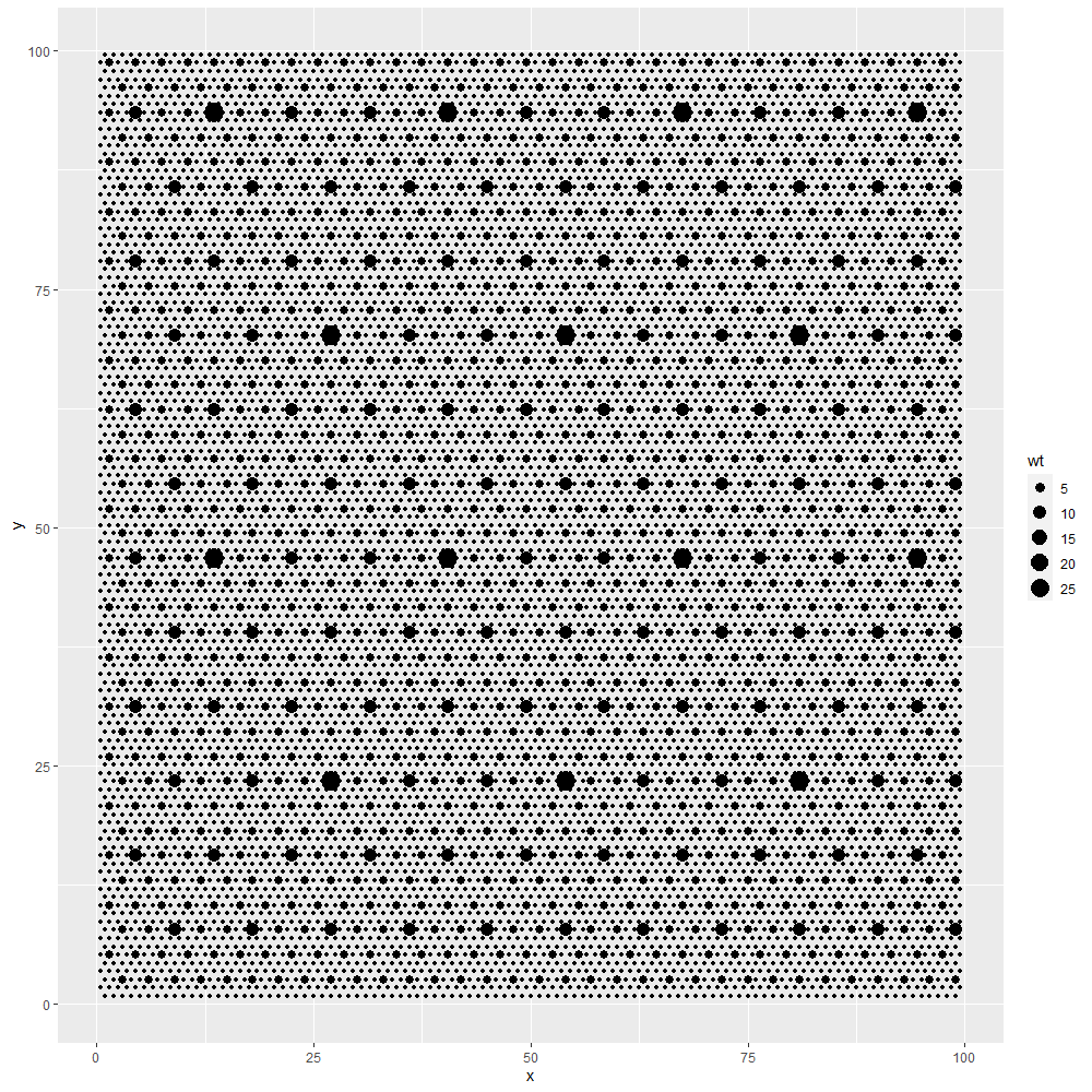
Trees semi-randomly planted at 1500 per 16 ha (and crowns of 10 m in diameter), simulating crown competition, cover 66.2% of the area, intermediate between the formula’s predicted 52.1% and the maximum potential area of 73.6%.
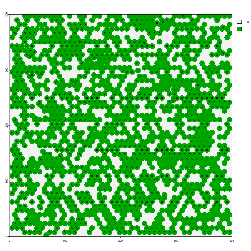
For most natural settings, when the only a few cover values are to be aggregated and for which there is a big difference in cover, the default formula by vegnasis::cover.agg() is adequate. But other applications where the need is to predict the total cover of multiple individuals competing in the same stratum, an alternative formulation by vegnasis::cover.agg.stratum() is given which averages the expected sum (maximum capped at 100%) and the default formula.